Toronto Blue Jays Attendance
Authors
- Gage Sonntag
- David Murray
Executive Summary
The work below was conducted in June 2017 as an extension of a Masters of Management Analytics course project offered by Queen’s University. The high-level goal of the project was to determine the various factors that contribute to ticket sales at Toronto Blue Jays home games. Specifically, we wanted to explore the following areas:
- To what degree does winning, both within a season and carryover from past years, help increase attendance?
- What sort of impact do certain types of promotions and giveaways have on attendance?
- What sort of attendance can be expected for the remainder of 2017 (July, August, September, October)?
Major findings include:
- With respect to winning:
- Making the playoffs the previous year has a much higher impact on total year attendance than good in-season performance (measured by games back variable)
- Win streaks of three and five were insignificant, but +5,000 fans are expected on average when the Jays have won seven games in a row
- With respect to promotions:
- Bobblehead giveaways typically increase attendance by between 1,000-4,000 fans per game
- With respect to predictive power:
- Our model was, on average, off by 8.8% per game through the first 28 games in 2017.
- In aggregate, our model predicted 1,030,640 fans in the first 28 games, and the actual was 1,052,390
- Jays forecasted attendance for 2017 under a simulated .500 performance the rest of the year is 3.34 million.
- As of June 2nd, total attendance for 2017 from June 2nd onwards is predicetd to be slightly below the 2016 total of 3.39 million.
- For games played at home between June 2nd and the end of July, our model has, on average, been off by 4.5% per game (not seen in report, but can compare Appendix 2 to Baseball Reference)
The Process
Data
- Scraped data from Baseball Reference
- Games scraped from 2004 to 2016, plus the first two months of 2017
- Binary variables added for whether Leafs/Raps were in playoffs
- Other data included Weather data from Stats Canada , Promotional Data from Jays, and Salary Cap Data from Sean Lahman’s Database.
- Some data cleaning was performed on the above datasets and then combined into a final dataset (Appendix 1)
- Baseball makes for easy statistical analysis both in the game, and for game attendance
Methodology
- Entire analysis conducted in R-Markdown
- Dataset containing ~1,000 games from 2004 to 2016
- With-held 75% of the observations to ‘train’ the model, and tested on the remaning 25%
- Used k-fold validation in machine learning models with ten folds
- All metrics shown are on test set data
- The model had never seen 2017 data before the testing
Feature Engineering
- Using the Date and Team variables in the final dataframe, we performed some feature engineering
- Games in a series GIS was created to track game number in the series
#Create Vector, set first game to 1
final$GIS<-as.numeric(vector(length=nrow(final)))
final$GIS[1] <- 1

#Step through games. If the team changes increment GIS. If the year changes, reset to 1.
for (i in 2:nrow(final)) {
     if (final$Team[i] != final$Team[i-1])
     {final$GIS[i] <- 1}
     else {final$GIS[i] <- final$GIS[i-1]+1}
}
rm(i)
- Home Opener was manufactured because of the baseball intuition that Jays games generally sell out in the first game of each season
#Engineer Season Opening Games
Opener <- final %>%
  group_by(Year) %>%
  summarise(Date=min(Date))
Opener<-data.frame(Opener)
final$Opener <- as.numeric(final$Date %in% Opener$Date)
- Other features aren’t shown but include:
- Series tracks series in the season (typically 26 home series per year)
- Late Season GB represents the number of Games Back the Jays may be in August, September or October, and was created to account for the possile added sensitivity of fans in these months
- Two Fourier terms (used in harmonic regression) were introduced and normalized to the length of the MLB season to capture any seasonality that would be expected
- Anecodatally, the Jays see a surge in popularity during the warm summer months when the dome is open and the schools are out
- This was added to allow any of the seasonal effects to be wrapped into 2 variables rather than 8 monthly variables
- Other variables include
- A Playoffs variable for whether the Jays made the playoffs in the previous season
- A Holiday variable for whether the game was played on an observed Canadian holiday
- A Streaks variable for whether the Jays have won 3, 5 or 7 games in a row
The Business Case
- Let’s look at how Attendance has changed since 2004
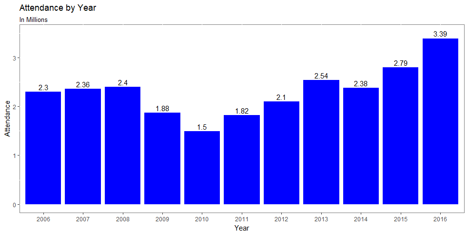
- The average ticket price in that span are shown below, the average for which was $24.6
- It’s important to note that the Jays rank tied for 18th in ticket prices, a far cry from the $52 average that the Boston Red Sox were charging in 2015

- We can extrapolate these prices to estimate total revenue from ticket sales over the past ten years (Average Ticket Price x Attendance)
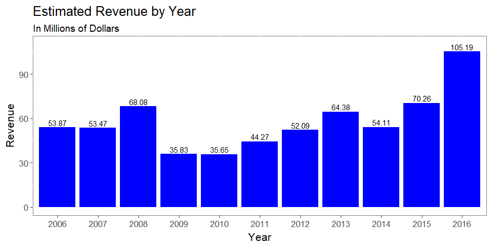
- The growth in revenue above is in some part driven by ticket prices, and otherwise driven by demand for those seats which is a business problem that, we believe, deserves further technical analysis
Descriptive Analytics
- From intuition, we know that the day of the game is likely to be important
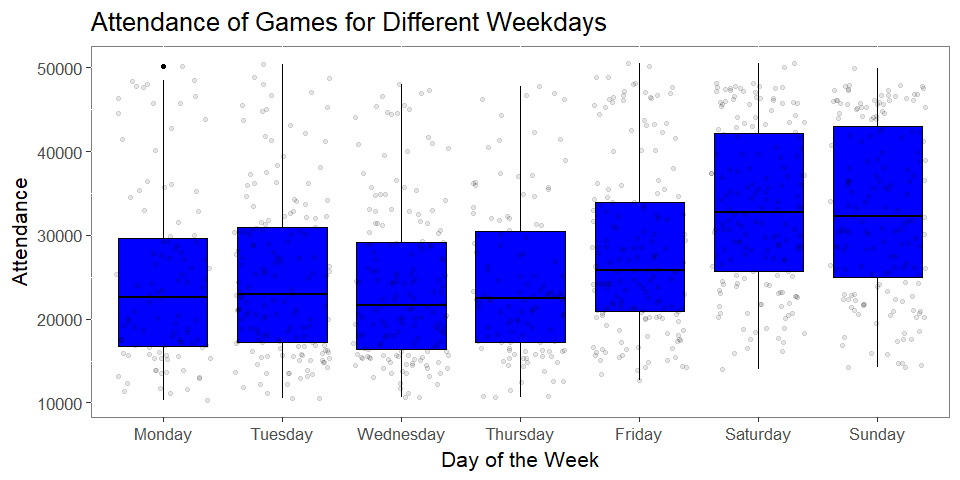
- Saturday and Sunday games, on average, tend to draw more fans than Weekday games
- Fridays capture some of this increased attendance as well
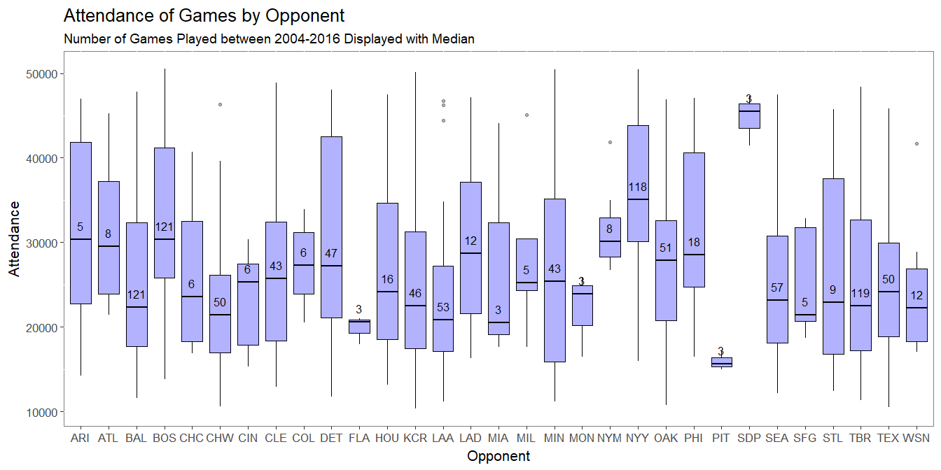
- We see considerable variation in attendance based on who they are playing
- However, over 30 teams are too many categories for the 1050 games in our sample
- Salary will help capture the effects of the big market teams
- BinRival will help to capture the increased attendance for Yankees and Red Sox Games
- A Proximity variable for opposing teams that are within a short drive to Toronto and may attract fans.
#Create binary variable for NYY, BOS
final<-final%>%
  mutate(BinRival=Team %in% c("BOS","NYY"))

#Proximity Variable for Driveable Distances
final<-final%>%
  mutate(Proximity=Team %in% c("CLE","CIN","NYY","CHC", "CWS","DET","PHI", "PIT"))
- We’ve seen the possible difference between opponents and within the week, now let’s look at different months in the season
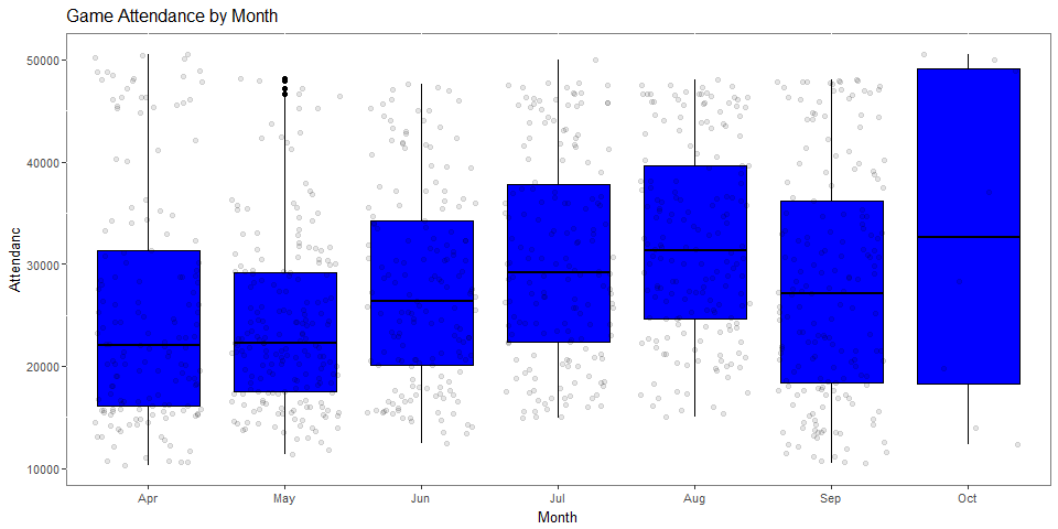
- We validate some of our intuition; April starts with a season opening bang, but after that it tapers off
- People like to see the Jays when the dome is open in the hot summer months of July and August
- Attendance may taper off or grow as the season draws to a close, likely based on team performance
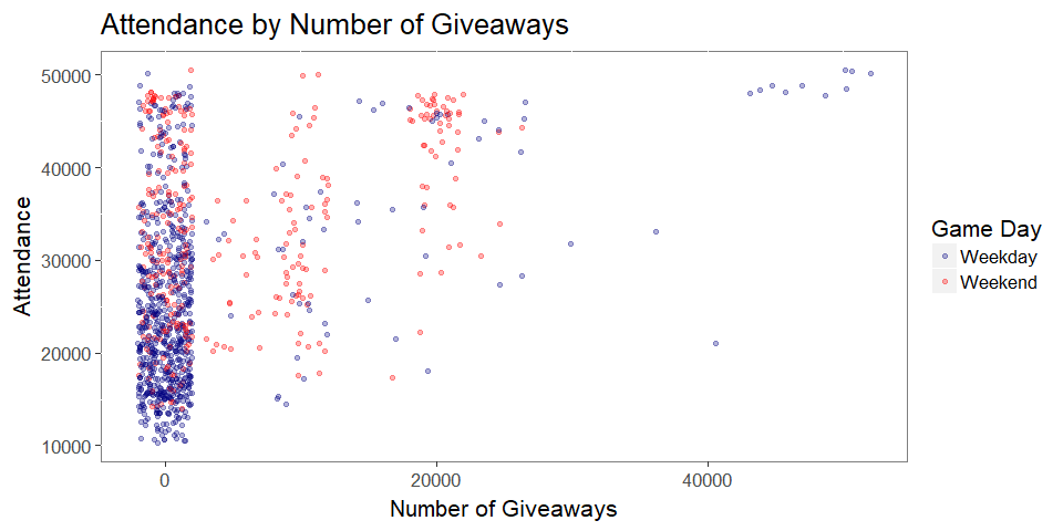
- We can see that there is some correlation between increased attendance as the number of promo giveaways increases
- However, we know that the 50k promo giveaway games were for a home openers and home opening series
- As well, we can see that most of the 20,000 giveaway games were on the weekend
- Let’s look deeper at bobblehead giveaways, one that we think would have the highest effect on Attendance
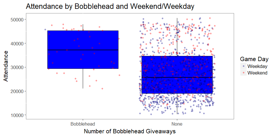
- At first glance, the effect of a promotion like the bobblehead figurines is significant
- However, most of the games are on weekends, so this is likely a confounding effect
- We will need our regression model to consider these other factors to tease out what’s really going on
Modeling
- In this project, we used a number of complex algorithms to predict attendance for 2017
- Random Forest
- Gradient Boosted Machine
- Deep Learning in h2o
- We also experimented with some easier-to-understand models. They include:
- Censored Regression
- Standard OLS Regression with Fourier terms using intuition and stepwise selection
- Combination of logistic regression (to predict sellout) and OLS regression
- For the purposes of this demonstration, we have shown the best “black box” model for predictive power (Random Forest), and the best “white box” option for inferring about factors that affect attendance (Stepwise OLS Regression)
Blackbox
- For this sort of problem, Random Forest looks attractive because it:
- Captures complex interactive relationships between variables
- Handles extraneous information well
- Has shown good success on Kaggle
- Will not predict outside the domain of given response variables
- In layman terms, this means it will not predict attendance over 50,000 for any game, where almost all other models would do this
#Set Model Seeds

set.seed(42)
seeds <- vector(mode = "list", length = 11)
for(i in 1:10) {seeds[[i]]<- sample.int(n=100000, 10)}
seeds[[11]] <- sample.int(n=100000,1)
rm(i)

#Set Parallel Computing
cl = makeCluster(2)
registerDoParallel(cl)

#Set caret parameters
kfolds=10
search.length=10

cvCtrl <- trainControl(method="cv",
                       number=kfolds,
                       seeds=seeds)

forest <- train(Attendance~.,
                method="rf",
                trControl=cvCtrl,
                data=final_train,
                importance=TRUE,
                tuneLength=search.length)

stopCluster(cl)
remove(cl)
registerDoSEQ()
## rf variable importance
##
##   only 20 most important variables shown (out of 58)
##
##              Overall
## Year          100.00
## Salary         77.47
## cosT           41.96
## Game           40.98
## Series         37.98
## GB             37.57
## sinT           36.93
## BinaryDay      36.64
## PromoAmount    36.39
## BinRivalTRUE   35.19
## Playoffs       34.16
## DayN           33.24
## DayNum         32.55
## MinTemp        25.90
## Rank           25.74
## LateSeasonGB   24.87
## MeanTemp       23.55
## Opener         22.09
## MonthNum       20.11
## Weekend1       19.46

## [1] "The MAPE of the random forest is 14.72 %"
- The MAPE (average percent error) suggests reasonably good predictive power
- Date was the most significant variable, likely because it captures the recent success of the Jays
- PromoAmount, or the number of giveaways at a game, proved to be a good predictor for attendance
When is our Predictive (Blackbox) Model Wrong?
- Lets begin to explore when the model is wrong, to understand if there are systemic inaccuracies.
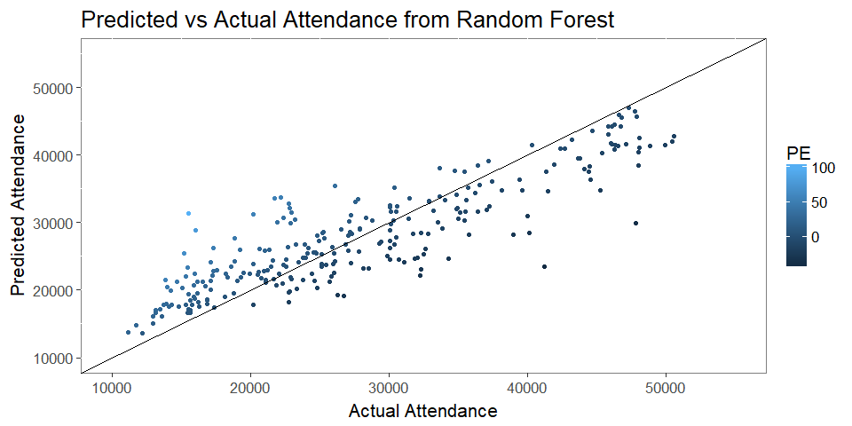
- A perfect estimator would have all data points fall along the line on the figure.
- Our forest appears to have over-optimistic estimates for low attended games, while when the games are popular, it tends to be too conservative, which isn’t a bad trait for a forecasting tool.
- Let’s use a simpler model to gain insight into Attedance drivers
Whitebox Model (Stepwise OLS Regression)
- This Stepwise OLS Regresion was built to satisfy course requirements.
- It selects only statistically significant variables at the p=0.10 level to include in the model.
##
## Call:
## lm(formula = Attendance ~ sinT + cosT + Salary + Day + Playoffs +
##     PromoAmount + Weekday + Rank + Opener + Series + GB + BinRival +
##     Streak7 + Bag + Leafs + Raps + Holiday + Figurine + OtherWear +
##     MinTemp + Hat + LateSeasonGB + GIS, data = step_train)
##
## Residuals:
##    Min     1Q Median     3Q    Max
## -17831  -3924   -354   3641  22840
##
## Coefficients:
##                    Estimate Std. Error t value Pr(>|t|)
## (Intercept)       2.448e+04  2.206e+03  11.096  < 2e-16 ***
## sinT             -1.310e+03  5.073e+02  -2.582  0.01000 *
## cosT             -2.523e+03  5.656e+02  -4.461 9.37e-06 ***
## Salary            4.962e+02  6.597e+01   7.522 1.53e-13 ***
## DayN             -5.996e+03  1.029e+03  -5.828 8.27e-09 ***
## Playoffs          9.793e+03  9.047e+02  10.825  < 2e-16 ***
## PromoAmount       2.585e-01  4.474e-02   5.776 1.11e-08 ***
## WeekdayTuesday    2.356e+03  9.095e+02   2.591  0.00976 **
## WeekdayWednesday  1.641e+03  9.955e+02   1.648  0.09970 .
## WeekdayThursday   1.801e+03  1.090e+03   1.652  0.09892 .
## WeekdayFriday     4.467e+03  9.039e+02   4.941 9.55e-07 ***
## WeekdaySaturday   5.728e+03  1.278e+03   4.481 8.56e-06 ***
## WeekdaySunday     1.734e+03  1.383e+03   1.254  0.21039
## Rank             -6.828e+02  2.808e+02  -2.432  0.01526 *
## Opener            1.608e+04  2.787e+03   5.771 1.15e-08 ***
## Series            5.153e+02  6.927e+01   7.439 2.75e-13 ***
## GB               -1.730e+02  8.921e+01  -1.939  0.05291 .
## BinRivalTRUE      3.925e+03  8.190e+02   4.792 1.99e-06 ***
## Streak7           5.160e+03  1.820e+03   2.836  0.00469 **
## Bag              -2.885e+03  1.626e+03  -1.774  0.07643 .
## Leafs             3.473e+03  1.363e+03   2.548  0.01104 *
## Raps              2.332e+03  1.104e+03   2.112  0.03505 *
## Holiday           3.357e+03  1.620e+03   2.072  0.03856 *
## FigurineNone     -3.643e+03  1.315e+03  -2.771  0.00572 **
## OtherWear         4.748e+03  1.917e+03   2.477  0.01347 *
## MinTemp          -1.242e+02  6.738e+01  -1.844  0.06561 .
## Hat               3.868e+03  1.891e+03   2.046  0.04108 *
## LateSeasonGB     -1.474e+02  7.962e+01  -1.851  0.06460 .
## GIS              -6.079e+02  3.737e+02  -1.627  0.10417
## ---
## Signif. codes:  0 '***' 0.001 '**' 0.01 '*' 0.05 '.' 0.1 ' ' 1
##
## Residual standard error: 6101 on 760 degrees of freedom
## Multiple R-squared:  0.6759, Adjusted R-squared:  0.664
## F-statistic: 56.61 on 28 and 760 DF,  p-value: < 2.2e-16

## [1] "The MAPE of the OLS Regression is 18.49"
- We removed Year, Month and Date variables in our model and they are replaced by the sinT & cosT variables for time
- This was done to maintain the model’s effectiveness at predicting 2018 season games
- MAPE (average percent error) of ~18% suggests mediocre predictive power:
- Oddly, when the Leafs are in the playoffs on the same day, they have a positive effect on game attendance. This is a very unintuitive result.
- When the Jays hit a 7 game streak, they experience an attendance boost of 6,000.
- For every additional $10M in opposing team Salary, 430 more people are interested in the game.
- The Jays made the playoffs in 2016 so, everything else equal, the Jays should expect an incremental 10,000 fans in 2017 as well.
- The negative effects of GB and the Jays Rank in their division coincide with our belief that winning affects the number of fans that come to games.
- The negative coefficients imply that total Attendance is affected by -670 (for each additional Rank) and -230 (for each additional GB)
- Late in the season, 140 less fans come to games for each additional game back, on top of 230 previously mentioned
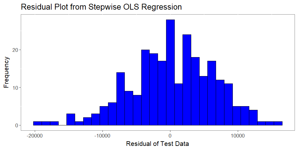 We see that our residuals are reasonably normal, with some fairly significant outliers.
2017 Predictions
- One of the goals of this project was to determine attendance for the rest of 2017 and to predict whether a repeat of 2016 attendance could occur, while factoring in the first 28 games of the 2017 season.
First 28 Games
- At the time of testing, the first 28 games up to and including the June 1st game against NYY had occurred
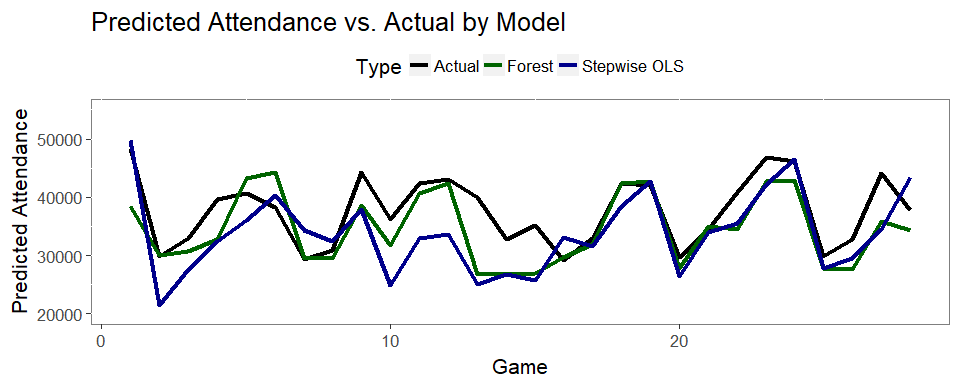
- Let’s look at how each model performs on the new holdout data
| Stepwise OLS Regression | Random Forest | |
|---|---|---|
| Model_MAPE | 14.10 | 9.74 |
| Model_RMSE | 6355.81 | 5045.26 |
- Here’s a plot to see how each model predicted each game, vs. the actual
- Take special note of Game 9, which is when actual attendance was significantly higher than each model predicted
- This was Edwin Encarnacion’s first game back to Toronto as a Cleveland baseball player - Something no model would be able to predict!
Predictions for Remaining Games
- First, let’s review what total attendance has done the past five seasons.
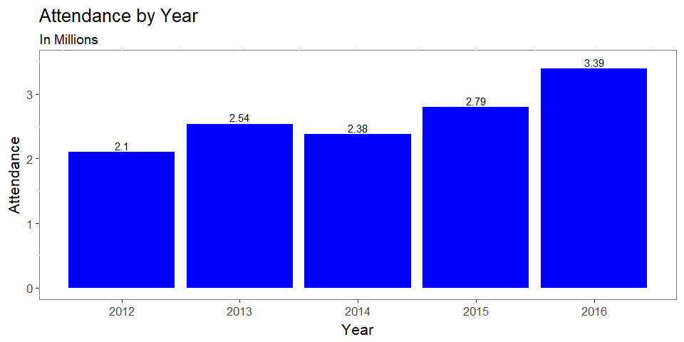
- The Jays may be interested to see if this trend will reverse in 2017.
- We used the random forest model to predict the remaining Jays games under three performance scenarios for the Jays:
- Bad performance (Rank 5th in AL East, and stay 12 games back for duration of 2017)
- Medium performance (Rank 3rd in AL East, and stay 7 games back for duration of 2017)
- Good performance (Rank 2nd in AL East, and stay 2 games back for duration of 2017)
#First let's create the datasets for the remaining 53 games
BadRemain <- Remaining2017 %>%
  mutate(Rank = 5,
         GB = 12,
         MaxTemp = mean(final_train$MaxTemp),
         MinTemp = mean(final_train$MinTemp),
         MeanTemp = mean(final_train$MeanTemp),
         LateSeasonGB = ASO * GB)

MediumRemain <- Remaining2017 %>%
  mutate(Rank = 3,
         GB = 7,
         MaxTemp = mean(final_train$MaxTemp),
         MinTemp = mean(final_train$MinTemp),
         MeanTemp = mean(final_train$MeanTemp),
         LateSeasonGB = ASO * GB)

GoodRemain <- Remaining2017 %>%
  mutate(Rank = 1,
         GB = 2,
         MaxTemp = mean(final_train$MaxTemp),
         MinTemp = mean(final_train$MinTemp),
         MeanTemp = mean(final_train$MeanTemp),
         LateSeasonGB = ASO * GB)

#lets build a list and predict on them.
scenarios <- list(BadRemain, MediumRemain, GoodRemain)
preds_list <- lapply(scenarios, function(x){predict(forest, x)})
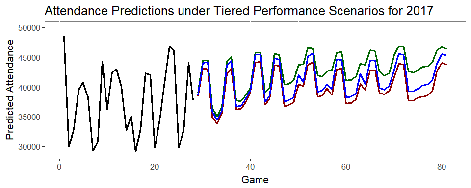
- As you can see, the model predicts very little variation in expected attendance depending on performance
- Interestingly, (and luckily for the Jays as of the end of July), the difference in Attendance between Good and Medium performance is much higher (53,000) than between Medium and Bad performance (24,000)
- While the higher late season attendance seems suspect compared to earlier games, our descriptive analytics showed a large uptick in attendance for late season games
- The Jays are lucky in that 9 of the remaining 17 series are to be played on Weekends
- Two of those 8 weekday series are played against NYY or BOS, games that typically do well regardless of day
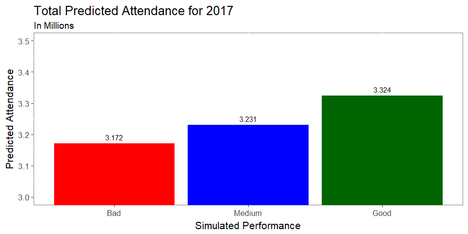
- Total attendance for 2017, even under poor performance, is expected to be 3.37 million
- It should be noted that other models had “Bad” performance around the high 3.2s, a much more realisitic estimate
- The associated revenue for Bad performance, assuming an average ticket price of $33.5 is $110 million
Next Steps
- Operationally, a model like this would help to predict 2018 attendance
- To do so, with the Jays unlikely to make the playoffs (as of end of July 2017), we would seek to expand the domain of our training dataset to include seasons where the Jays were coming off two straight playoff berths (1995)
- Theoretically, these models could provide confidence intervals for each game
- Executives could test the impact that a given promotion may have against a null hypothesis
- Is the cost of promotion XYZ really worth it? How many more fans did it bring in?
- The model could be used to negotiate scheduling with both stadium owners and the MLB
- Questions like the following could be answered
- Are we better to play the Rays or the Orioles on a Weekday series?
- When should we schedule our promotions?
- Additional information could be added to the model
- How do lower-bowl tickets sell relative to upper-bowl against the Yankees?
- Are fans more price sensitive for in-demand games or tertiary games?
- Dashboards could be built for executives that update with forecasts after every home game played, for the duration of the year
- Similar methodology could be applied in tandem with concession sales to help catering services better serve customers
If you’re interested in learning more about the work that was done, please contact David Murray or Gage Sonntag.
Appendix
- The following is the ‘structure’ of the dataset used to predict attendance:
Structure of Dataset Used
## 'data.frame':    1050 obs. of  49 variables:
##  $ Game           : int  1 2 3 10 11 12 13 14 15 26 ...
##  $ Attendance     : num  47817 21003 13100 14239 20177 ...
##  $ Leafs          : int  1 1 1 0 1 1 1 1 1 1 ...
##  $ Raps           : int  0 0 0 0 0 0 0 0 0 0 ...
##  $ Rank           : num  4 5 5 5 5 5 5 5 5 5 ...
##  $ GB             : num  1 1.5 2 2.5 3.5 4.5 5.5 6 5.5 7.5 ...
##  $ Day            : Factor w/ 2 levels "D","N": 1 2 2 2 1 1 2 2 2 2 ...
##  $ Streak         : num  0 -1 -2 1 -1 -2 -3 -4 -5 -1 ...
##  $ BinaryDay      : num  1 0 0 0 1 1 0 0 0 0 ...
##  $ Year           : num  2004 2004 2004 2004 2004 ...
##  $ Month          : Factor w/ 7 levels "Apr","May","Jun",..: 1 1 1 1 1 1 1 1 1 2 ...
##  $ MaxTemp        : num  2.5 7.4 9.9 12.8 18.4 11.6 8.7 17.2 15.3 9.4 ...
##  $ MinTemp        : num  -6.2 -2.7 3.1 4.8 6.9 7.9 4.3 5.8 8.5 1.6 ...
##  $ MeanTemp       : num  -1.9 2.4 6.5 8.8 12.7 9.8 6.5 11.5 11.9 5.5 ...
##  $ Precipitation  : num  0 3.8 0 0 3.4 10.6 0 11.8 0 0 ...
##  $ Salary         : num  4.68 4.68 4.68 5.16 5.16 ...
##  $ Hat            : num  0 0 0 0 0 0 0 0 0 0 ...
##  $ Jersey         : num  0 0 0 0 0 0 0 0 0 0 ...
##  $ Shirt          : num  0 0 0 0 0 0 0 0 0 0 ...
##  $ Figurine       : Factor w/ 2 levels "Bobblehead","None": 2 2 2 2 2 2 2 2 2 2 ...
##  $ Bag            : num  0 0 0 0 0 0 0 0 0 0 ...
##  $ OtherWear      : num  0 0 0 0 0 0 0 0 0 0 ...
##  $ NonWear        : num  1 1 0 0 1 0 0 0 0 0 ...
##  $ Kids           : num  0 0 0 0 0 0 0 0 0 0 ...
##  $ PromoAmount    : num  50000 40000 0 0 10000 0 0 0 0 0 ...
##  $ KidsTheme      : num  0 0 0 0 0 0 0 0 0 0 ...
##  $ AdultTheme     : num  0 0 0 0 0 0 0 0 0 0 ...
##  $ GIS            : num  1 2 3 1 2 3 1 2 3 1 ...
##  $ Opener         : num  1 0 0 0 0 0 0 0 0 0 ...
##  $ Holiday        : num  0 0 0 0 0 0 0 0 0 0 ...
##  $ Playoffs       : num  0 0 0 0 0 0 0 0 0 0 ...
##  $ BinaryPrecip   : num  0 1 0 0 1 1 0 1 0 0 ...
##  $ Weekday        : Factor w/ 7 levels "Monday","Tuesday",..: 1 2 3 5 6 7 2 3 4 1 ...
##  $ MonthNum       : num  4 4 4 4 4 4 4 4 4 5 ...
##  $ DayNum         : num  1 2 3 5 6 7 2 3 4 1 ...
##  $ sinT           : num  0 0.0347 0.0694 0.3726 0.4046 ...
##  $ cosT           : num  1 0.999 0.998 0.928 0.914 ...
##  $ Series         : num  1 1 1 2 2 2 3 3 3 4 ...
##  $ ASO            : num  0 0 0 0 0 0 0 0 0 0 ...
##  $ Streak7        : num  0 0 0 0 0 0 0 0 0 0 ...
##  $ Streak5        : num  0 0 0 0 0 0 0 0 0 0 ...
##  $ Streak3        : num  0 0 0 0 0 0 0 0 0 0 ...
##  $ JunJul         : num  0 0 0 0 0 0 0 0 0 0 ...
##  $ AprMay         : num  1 1 1 1 1 1 1 1 1 1 ...
##  $ LateSeasonGB   : num  0 0 0 0 0 0 0 0 0 0 ...
##  $ Weekend        : Factor w/ 2 levels "0","1": 1 1 1 1 2 2 1 1 1 1 ...
##  $ Weekday_Daytime: num  0 0 0 0 1 1 0 0 0 0 ...
##  $ BinRival       : logi  FALSE FALSE FALSE FALSE FALSE FALSE ...
##  $ Proximity      : logi  TRUE TRUE TRUE FALSE FALSE FALSE ...
Predictions for Remainder of Year
- For comparison: Baseball Reference 2017
| Date | Opponent | Weekday | Bad | Medium | Good |
|---|---|---|---|---|---|
| 2017-06-02 | NYY | Friday | 38363 | 38616 | 38974 |
| 2017-06-03 | NYY | Saturday | 43157 | 44085 | 44474 |
| 2017-06-04 | NYY | Sunday | 43015 | 44139 | 44432 |
| 2017-06-13 | TBR | Tuesday | 34994 | 35907 | 36527 |
| 2017-06-14 | TBR | Wednesday | 33873 | 34413 | 34982 |
| 2017-06-16 | CHW | Friday | 35610 | 36051 | 36720 |
| 2017-06-17 | CHW | Saturday | 42278 | 43524 | 44327 |
| 2017-06-18 | CHW | Sunday | 43023 | 44464 | 45095 |
| 2017-06-27 | BAL | Tuesday | 36250 | 36750 | 37713 |
| 2017-06-28 | BAL | Wednesday | 36301 | 36821 | 37621 |
| 2017-06-29 | BAL | Thursday | 37567 | 38097 | 38703 |
| 2017-06-30 | BOS | Friday | 39173 | 39430 | 39839 |
| 2017-07-01 | BOS | Saturday | 44145 | 45418 | 45766 |
| 2017-07-02 | BOS | Sunday | 44249 | 45475 | 45805 |
| 2017-07-06 | HOU | Thursday | 36939 | 37547 | 39022 |
| 2017-07-07 | HOU | Friday | 38056 | 38464 | 39862 |
| 2017-07-08 | HOU | Saturday | 43609 | 44757 | 45603 |
| 2017-07-09 | HOU | Sunday | 43515 | 44637 | 45399 |
| 2017-07-24 | OAK | Monday | 36762 | 37581 | 40468 |
| 2017-07-25 | OAK | Tuesday | 36963 | 37780 | 40518 |
| 2017-07-26 | OAK | Wednesday | 37351 | 38192 | 41069 |
| 2017-07-27 | OAK | Thursday | 40394 | 42074 | 43721 |
| 2017-07-28 | LAA | Friday | 40203 | 40733 | 43795 |
| 2017-07-29 | LAA | Saturday | 43759 | 45108 | 46590 |
| 2017-07-30 | LAA | Sunday | 44100 | 45591 | 46455 |
| 2017-08-08 | NYY | Tuesday | 38336 | 39201 | 41910 |
| 2017-08-09 | NYY | Wednesday | 38565 | 39444 | 41721 |
| 2017-08-10 | NYY | Thursday | 39810 | 40466 | 42688 |
| 2017-08-11 | PIT | Friday | 38578 | 39706 | 42773 |
| 2017-08-12 | PIT | Saturday | 43011 | 44589 | 45780 |
| 2017-08-13 | PIT | Sunday | 43092 | 44578 | 45838 |
| 2017-08-14 | TBR | Monday | 37211 | 38177 | 41065 |
| 2017-08-15 | TBR | Tuesday | 37299 | 38334 | 41159 |
| 2017-08-16 | TBR | Wednesday | 37846 | 38904 | 41776 |
| 2017-08-17 | TBR | Thursday | 40524 | 42221 | 43849 |
| 2017-08-25 | MIN | Friday | 39508 | 40409 | 43692 |
| 2017-08-26 | MIN | Saturday | 42784 | 44483 | 46213 |
| 2017-08-27 | MIN | Sunday | 42809 | 44459 | 46016 |
| 2017-08-28 | BOS | Monday | 38960 | 39836 | 42532 |
| 2017-08-29 | BOS | Tuesday | 38770 | 39527 | 41897 |
| 2017-08-30 | BOS | Wednesday | 39390 | 40197 | 42290 |
| 2017-09-08 | DET | Friday | 41590 | 42901 | 45381 |
| 2017-09-09 | DET | Saturday | 43861 | 45523 | 46843 |
| 2017-09-10 | DET | Sunday | 43795 | 45448 | 46827 |
| 2017-09-11 | BAL | Monday | 37710 | 39279 | 42609 |
| 2017-09-12 | BAL | Tuesday | 37680 | 39255 | 42387 |
| 2017-09-13 | BAL | Wednesday | 38220 | 39719 | 42836 |
| 2017-09-19 | KCR | Tuesday | 38343 | 40282 | 43381 |
| 2017-09-20 | KCR | Wednesday | 38505 | 40435 | 43495 |
| 2017-09-21 | KCR | Thursday | 39376 | 41129 | 44231 |
| 2017-09-22 | NYY | Friday | 42611 | 43853 | 46107 |
| 2017-09-23 | NYY | Saturday | 44048 | 45494 | 46785 |
| 2017-09-24 | NYY | Sunday | 43681 | 45291 | 46340 |